This post aims to shine a light on the Convolutional Neural Network, the technology which underpins the amazing image recognition abilities of tech behemoths such as Facebook and Google and hints at the tremendous potential of artificial intelligence.
This post will use the 'hello world' of image recognition the database of handwritten digit images MNIST to describe the intricacies of the technique.
The network will take single channel grayscale MNIST images as input and be composed of 3 cross correlation filters feeding forward into 3 convolved images followed by a pool reducing the width and height of the input field by half followed lastly by a softmax layer. Cross entropy will be used as the error term. It will be shown how enormously successful this simple model is at image recognition.
The network will use stochastic gradient descent for learning and the learning rate parameter will be tuned using a combination of epochs on a sample of training and validation data sets.
The below image describes how the input image X is convolved with the filter f to produce the convolutions layer Y.

$$
\begin{align}
Y &= X \otimes f && [784 \times 3] \\
\text{ in other words:} \\
Y_{k}(i,j) &= \sum_{a=0}^{a=2} \sum_{b=0}^{b=2} X(i+a,j+b) f(a,b) \\
\end{align}
$$
The previous article highlighted how the weights evolved to specialise in exposing discriminating features in the input field. The convolution builds on this feature by incorporating a layer comprising multiple convolution filters each focusing on the aforementioned benefit of specialising in bringing forward discriminating features. An added benefit is that it introduces a hierarchy where a relationship is formed between adjacent weights in the same filter where these weights are forced to share the burden of identifying the relevant feature in that filter's input field discrimination specialisation. An added benefit is that it reduces the number of parameters in the model which drastically speeds up calculations.
The filters used in this case is a bank of 3 cross correlation kernels which extracts similar features to itself from the input field into a bank of 3 convolved images down the line for further processing.
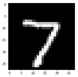
The below image is an example of an image in the MNIST training data set and is given the label '7' for model learning purposes.

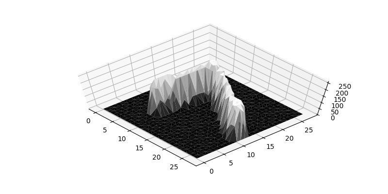
The below image is a 3d plot of the record.

The kernels used in this model's case, examples of which are shown below, are of dimension 3×3.

Similarly, the below images are 3d plots of the kernels. These kernels will be scanned over the input image to isolate matching features.

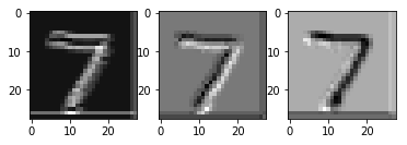
The below images are the convolved images of the input image. The peaks are white in colour and correspond to positions where the contours of the kernel correspond to the contours of the input image.


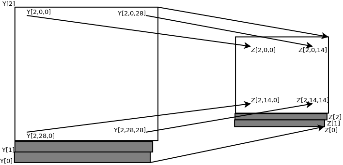
The image below describes the pooling layer that follows the convolution. It reduces the height and width of the input data field by half by simply letting every combination of even numbered pixels through to the next layer.

The pooling layer further reduces the number of parameters and calculations while maintaining the overall structure and linear invariance of the input data field.
$$
\begin{align}
Z_{k} (\frac{i}{2},\frac{j}{2}) = Y_{k}(i,j) && [196 \times 3]
\end{align}
$$

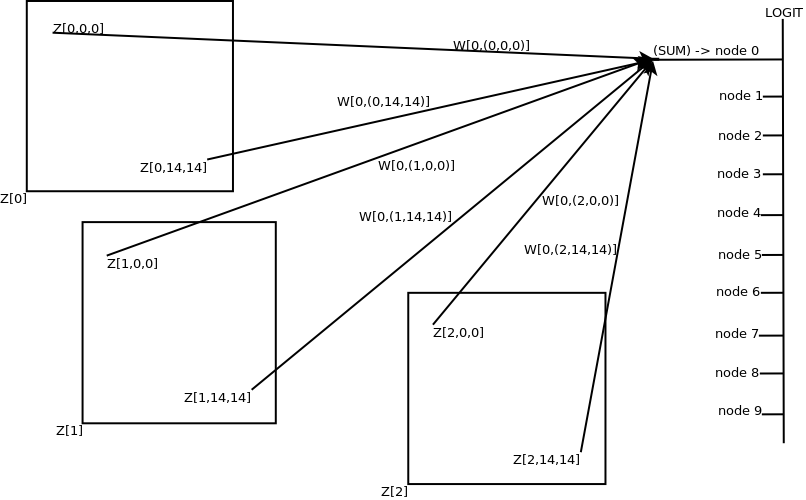
The learnings of the discriminating features and relationships between the weights are now aggregated into one of the output classes the model given the input field is asked to recognise.
$$
\begin{align}
A &= WZ && [10 \times 14^2\cdot 3][14^2 \cdot 3 \times 1] \\
& \text{or}&& [10 \times 1]
\end{align}
$$
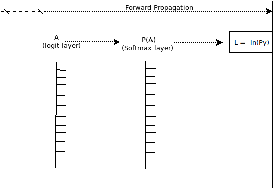
Softmax layer or probability the model estimates that the given output class is the correct classification for the input image.

$$
\begin{align}
P(A) &= \frac{e^{-a_j}}{\sum_{k=0}^{k=9} e^{-a_k}} && [10 \times 1]
\end{align}
$$
div>
$$
\begin{align}
L(P_{true},P) &= \sum_{i=0}^{i=9} P_{true,i} \ln P_i && [1 \times 1] \\
&= \ln P_y \\
\frac{\partial L}{\partial p} &= \left[ \frac {\partial L}{\partial p_0} \frac {\partial L}{\partial p_1} ... \frac {\partial L}{\partial p_9} \right] && [1 \times 10]\\
&= \left[0 ... \frac {\partial L}{\partial p_y} ... 0 \right]
\end{align}
$$
Derivation of the backward propogation phase:
$$
\begin{align}
\frac {\partial p}{\partial a} = \begin{bmatrix}
\frac{\partial p_1}{\partial a_1} & \frac{\partial p_1}{\partial a_2} & ... & \frac{\partial p_1}{\partial a_{9}} \\
\frac{\partial p_2}{\partial a_1} & \frac{\partial p_2}{\partial a_2} & ... & \frac{\partial p_2}{\partial a_{9}} \\
... & ... & ... & ... \\
\frac{\partial p_{9}}{\partial a_1} & \frac{\partial p_{9}}{\partial a_2} & ... & \frac{\partial p_{9}}{\partial a_{9}} \\
\end{bmatrix} && [10 \times 10]
\end{align}
$$
Let $$
\sum = \sum_{k=0}^{k=9} \\
$$
Then
$$
\begin{align}
\frac{\partial p}{\partial a}
= \begin{bmatrix}
\frac{e^{a_1}(\sum - e^{a_1})}{(\sum)^2} & -\frac{e^{a_1}e^{a_2}}{(\sum)^2} & ... & -\frac{e^{a_1}e^{a_9}}{(\sum)^2} \\
-\frac{e^{a_2}e^{a_1}}{(\sum)^2} & \frac{e^{a_2}(\sum - e^{a_2})}{(\sum)^2} & ... & -\frac{e^{a_2}e^{a_9}}{(\sum)^2} \\
... & ... & ... \\
-\frac{e^{a_9}e^{a_1}}{(\sum)^2} & -\frac{e^{a_9}e^{a_2}}{(\sum)^2} & ... & \frac{e^{a_9}(\sum - e^{a_9})}{(\sum)^2} \\
\end{bmatrix} && [10 \times 10]
\end{align}
$$
$$
\begin{align}
\frac{\partial L}{\partial a} &= \frac{\partial L}{\partial p} \frac{\partial p}{\partial a} &[1 \times 10][10 \times 10] && \text{or} && [1 \times 10]
\end{align}
$$
$$
\begin{align}
W && [10 \times (14^2 \cdot 3) ] \\
\end{align}
$$
Given that:
$$
\begin{align}
A_0 &= Z_{0,0,0}W_{0,0,0,0} + ... + Z_{0,14,14}W_{0,0,14,14} + Z_{1,0,0}W_{0,1,0,0} + ... + Z_{1,14,14}W_{0,1,14,14} + Z_{2,0,0}W_{0,2,0,0} + ... + Z_{2,14,14}W_{0,2,14,14} \\
A_1 &= Z_{0,0,0}W_{1,0,0,0} + ... + Z_{0,14,14}W_{1,0,14,14} + Z_{1,0,0}W_{1,1,0,0} + ... + Z_{1,14,14}W_{1,1,14,14} + Z_{2,0,0}W_{1,2,0,0} + ... + Z_{2,14,14}W_{1,2,14,14} \\
... \\
A_9 &= Z_{0,0,0}W_{9,0,0,0} + ... + Z_{0,14,14}W_{9,0,14,14} + Z_{1,0,0}W_{9,1,0,0} + ... + Z_{1,14,14}W_{9,1,14,14} + Z_{2,0,0}W_{9,2,0,0} + ... + Z_{2,14,14}W_{9,2,14,14}
\end{align}
$$
$$
\require{amsmath}
\require{mathtools}
\begin{align}
\frac{\partial A}{\partial W} =
\begin{bmatrix}
\overbrace{\overbrace{\frac{\partial A_0}{\partial W_{0,0,0,0}} ... \frac{\partial A_0}{\partial W_{0,0,14,14}}}^\text{img w deriv to class 0} \overbrace{\frac{\partial A_0}{\partial W_{1,0,0,0}} ... \frac{\partial A_0}{\partial W_{1,0,14,14}}}^\text{img w deriv to class 1} ... \frac{\partial A_0}{\partial W_{9,0,14,14}}}^\text{img w deriv for all of filter 0} \frac{\partial A_0}{\partial W_{0,1,0,0}} ... \frac{\partial A_0}{\partial W_{9,2,14,14}} \\
\frac{\partial A_1}{\partial W_{0,0,0,0}} ... \frac{\partial A_1}{\partial W_{0,0,14,14}} \frac{\partial A_1}{\partial W_{1,0,0,0}} ... \frac{\partial A_1}{\partial W_{1,0,14,14}} ... \frac{\partial A_1}{\partial W_{9,0,14,14}} \frac{\partial A_1}{\partial W_{0,1,0,0}} ... \frac{\partial A_1}{\partial W_{9,2,14,14}} \\
... ... ... ... ... ... ...... \\
\frac{\partial A_9}{\partial W_{0,0,0,0}} ... \frac{\partial A_9}{\partial W_{0,0,14,14}} \frac{\partial A_9}{\partial W_{1,0,0,0}} ... \frac{\partial A_9}{\partial W_{1,0,14,14}} ... \frac{\partial A_9}{\partial W_{9,0,14,14}} \frac{\partial A_9}{\partial W_{0,1,0,0}} ... \frac{\partial A_9}{\partial W_{9,2,14,14}} \\\
\end{bmatrix}
&& [10 \times (10 \cdot 14^2 \cdot 3)]
\end{align}
$$
$$
\require{amsmath}
\require{mathtools}
\begin{align}
\frac{\partial A}{\partial W} =
\begin{bmatrix}
Z_{0,0,0,0} & ... & Z_{0,0,14,14} & 0 & ... & 0 & ... & 0 & Z_{0,1,0,0} & ... & 0 \\
0 & ... & 0 & Z_{1,0,0,0} & ... & Z_{1,0,14,14} & ... & 0 & 0 & ... & 0 \\
... & ... & ... & ... & ... & ... & ... & ... & ... & ... & ... \\
0 & ... & 0 & 0 & ... & 0 & ... & Z_{9,0,14,14} & 0 &... & Z_{9,2,14,14} \\\
\end{bmatrix}
\\ [10 \times (10 \cdot 14^2 \cdot 3)]
\end{align}
$$
$$
\begin{align}
\frac {\partial L}{\partial W} &= \frac{\partial L}{\partial A}\frac{\partial A}{\partial W} && [1 \times 10][10 \times (10 \cdot 14^2 \cdot 3)] \\ &or&& [1 \times (10 \cdot 14^2 \cdot 3)]
\end{align}
$$
$$
\begin{align}
\frac{\partial A}{\partial Z} &&[10 \times (14^2 \cdot 3)]
\end{align}
$$
$$
\begin{bmatrix}
\frac{\partial A_0}{\partial Z_{0,0,0}} ... \frac{\partial A_0}{\partial Z_{0,14,14}} \frac{\partial A_0}{\partial Z_{1,0,0}} ... \frac{\partial A_0}{\partial Z_{1,14,14}} \frac{\partial A_0}{\partial Z_{2,0,0}} ... \frac{\partial A_0}{\partial Z_{2,14,14}} \\
\frac{\partial A_1}{\partial Z_{0,0,0}} ... \frac{\partial A_1}{\partial Z_{0,14,14}} \frac{\partial A_1}{\partial Z_{1,0,0}} ... \frac{\partial A_1}{\partial Z_{1,14,14}} \frac{\partial A_1}{\partial Z_{2,0,0}} ... \frac{\partial A_1}{\partial Z_{2,14,14}} \\
........................................ \\
\frac{\partial A_9}{\partial Z_{0,0,0}} ... \frac{\partial A_9}{\partial Z_{0,14,14}} \frac{\partial A_9}{\partial Z_{1,0,0}} ... \frac{\partial A_9}{\partial Z_{1,14,14}} \frac{\partial A_9}{\partial Z_{2,0,0}} ... \frac{\partial A_9}{\partial Z_{2,14,14}} \\
\end{bmatrix}
$$
$$
\begin{bmatrix}
W_{0,0,0,0} & \ldots & W_{0,0,14,14} & W_{0,1,0,0} & \ldots & W_{0,1,14,14} & W_{0,2,0,0} & \ldots & W_{0,2,14,14} \\
W_{1,0,0,0} & \ldots & W_{1,0,14,14} & W_{1,1,0,0} & \ldots & W_{1,1,14,14} & W_{1,2,0,0} & \ldots & W_{1,2,14,14} \\
\vdots&\ddots&\ddots&\ddots&\ddots&\ddots & \ddots & \ddots & \vdots \\
W_{9,0,0,0} & \ldots & W_{9,0,14,14} & W_{9,1,0,0} & \ldots & W_{9,1,14,14} & W_{9,2,0,0} & \ldots & W_{9,2,14,14} \\
\end{bmatrix}
$$
$$
\begin{align}
\frac{\partial L}{\partial Z} = \frac{\partial L}{\partial A}\frac{\partial A}{\partial Z} && [1 \times 10][10 \times (14^2 \cdot 3)] \\ && [1 \times (14^2 \cdot 3)]
\end{align}
$$
Given that:
$$X \otimes F = Y \\
\begin{bmatrix}
x_{0,0} & x_{0,1} & x_{0,2} & x_{0,3} \\
x_{1,0} & x_{1,1} & x_{1,2} & x_{1,3} \\
x_{2,0} & x_{2,1} & x_{2,2} & x_{2,3} \\
x_{3,0} & x_{3,1} & x_{3,2} & x_{3,3} \\
\end{bmatrix}
\otimes
\begin{bmatrix}
f_{0,0} & f_{0,1} & f_{0,2} \\
f_{1,0} & f_{1,1} & f_{1,2} \\
f_{2,0} & f_{2,1} & f_{2,2} \\
\end{bmatrix}
=
\begin{bmatrix}
y_{0,0} & y_{0,1} & y_{0,2} & y_{0,3} \\
y_{1,0} & y_{1,1} & y_{1,2} & y_{1,3} \\
y_{2,0} & y_{2,1} & y_{2,2} & y_{2,3} \\
y_{3,0} & y_{3,1} & y_{3,2} & y_{3,3} \\
\end{bmatrix}
$$
By the chain rule:
$$
\begin{align}
\frac{\partial L}{\partial f_{i,j}} &=\sum_{m=0}^{m=27} \sum_{n=0}^{n=27} \frac{\partial L}{\partial Y_{m,n}}\frac{\partial Y_{m,n}}{\partial f_{i,j}}
\end{align}
$$
$$
\begin{align}
Y_{m,n} &= \sum_{i'} \sum_{j'} X_{m+i',n+j'} f_{i',j'}
\end{align}
$$
$$
\begin{align}
&&= X_{m+0,n+0}f_{0,0} + \ldots + X_{m+i',n+j'}f_{i',j'}
\end{align}
$$
$$
\frac{\partial Y_{m,n}}{\partial f_{i,j}} = \frac{\partial}{\partial f_{i,j}}(x_{m+0,n+0}f_{0,0} + \ldots + x_{m+i,n+j}f_{i,j} + \ldots)
$$
which simplifies to $$
\frac{\partial Y_{m,n}}{\partial f_{i,j}} = \frac{\partial}{\partial f_{i,j}}( x_{m+i,n+j}f_{i,j} ) = x_{m+i,n+j}
$$
where $$i' = i$$ and $$j'=j$$ as the partial derivatives of all the other terms reduces to zero.
$$
\therefore
\begin{align}
\frac{\partial L}{\partial f_{i,j}} =\sum_{m=0}^{m=27} \sum_{n=0}^{n=27} \frac{\partial L}{\partial Y_{m,n}}X_{m+i,n+j}
\end{align}
$$
Results:
The simple convolutional neural network in this case is an example of a supervised model because it is fed with training data which provides the correct output class the fully evolved model is expected to predict given the relevant input data. This model uses a combination of a learning rate applied to its weights and filters, a set of training data and a certain number of training epochs which need to be carefully tuned to achieve the end of correctly classifying its input field. The learning rate is used to cautiously step the weights in possibly the correct direction of the ideal solution space.
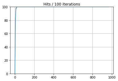
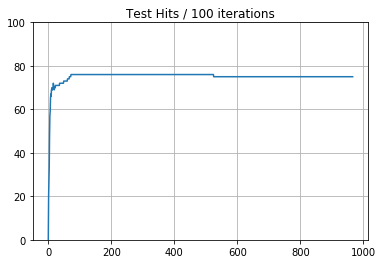
An example model specifically produced to demonstrate overtraining is presented in the plots above. The upper plot uses the training data as input whereas the lower plot uses the validation data as input. The plots are of the accuracy on the model per training epoch of 100 records. The model was trained on the training data for a total for 1000 epochs with the validation data set kept aside to display the generalising ability of the model.
The plots show that the model is able to correctly predict the output class with 100% accuracy very early on in its training whereas the validation plot shows that the model has poor image recognition capabilities, never reaching 80% and gradually deteriorating later on in the training cycle.

